MCHyper Tutorial:
MCHyper is a model checker for HyperLTL (a temporal logic able to express hyperproperties like noninterference) that builds on standard verification techniques from hardware model checking. Thus, it is used to verify a system against a hyperproperty relating multiple system traces. In the following, we introduce you to MCHyper and its interactive online tool interface.
The layout of the tool consists of three main sections:
Input,
Output
and
Console. In the Input
section, the input of the tool (system, property, options, ...) can be specified. When running the tool
with the
specified input, the result and some statistics are shown in the
Console. The
generated files
appear in the Output section when the tool finished.


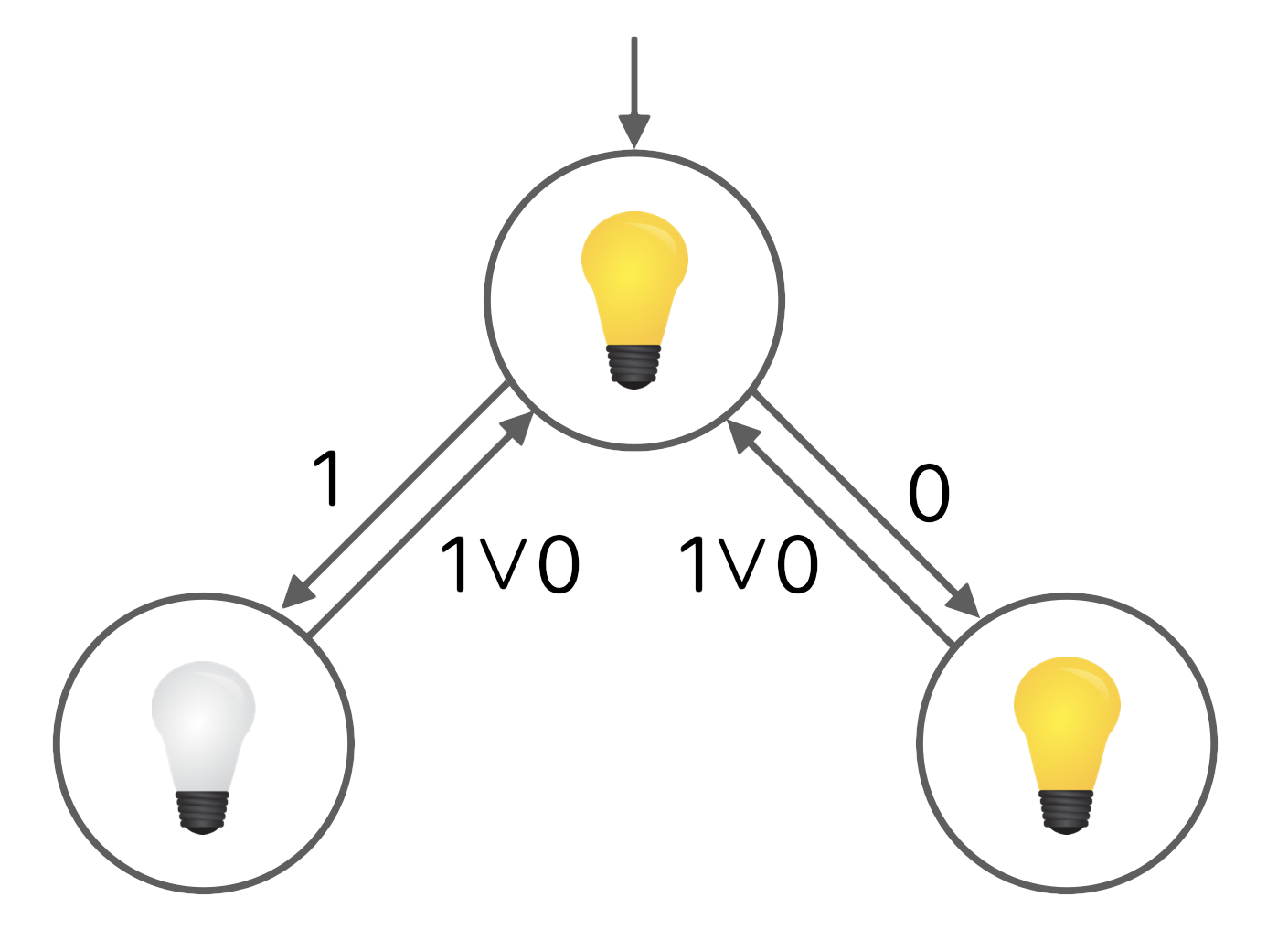
Let's assume we have a reactive system, that let us control a light with an input of zeros and ones. Additionally, we want our system to fulfill a certain property that ensures that the system works as expected.
First, let's focus on the Input section to specify the
above mentioned
example.
Specifying the system
First, we need to have a model of a system that we want to fulfill a property. Let's turn our attention to the following automaton representing our given system.
As specification language, MCHyper supports both Verilog and
Aiger (both are hardware description languages to model
circuits).
To specify the
automaton, you
can use the System tab in
the interface. The language (Verilog or Aiger) is inferred
automatically
while typing. In Verilog, our automaton can be realized as
follows:
Passing the hierarchical path name of the clock identifier (called "clock path") can be done under
Options in the Input section. For
example, the clock path for the module above is light/clock.
The clock path is inferred automatically if the clock identifier is clock, clk or c.
Let's understand why the above Verilog circuit mathes the
desired automaton. In our module, we keep track of the
current state in the state register. The
constant STATE_0 refers to the start state,
STATE_1 refers to the right state and
STATE_2 to the left. In the register
l we remember if the light is currently
ON or OFF and assign this value
to the output light. On
every clock tick, we change the state and the light
register depending
on the current state and the input given
in the in parameter just like the underlaying
automaton specifies it.
Since MCHyper only supports Aiger as input, the system
specified in Verilog is
converted to Aiger before using the tool Yosys (with the
flags -p "proc; techmap -map +/dff2ff.v; delete CLOCK_PATH; synth; aigmap; write_aiger -ascii -symbols" where CLOCK_PATH is replaced by the actual clock path)
and is then passed to MCHyper. To
skip this preprocessing step or use other flags to create
the Aiger circuit from the Verilog code, you
can directly enter the system in Aiger. For the sake of
completeness, this is the generated Aiger code for the above
specified
system:
Specifying the Property
Now we need to specify the property that should hold for the
system: for all possible input streams the light must
behave in the same
way. To specify the HyperLTL formula that describes the
property,
we use the
Formula tab in the Input section. In
our case, we state that for
every pair of
traces, the light should always behave the same way over the
whole trace:
This formula is written in the
EAHyper input format. The grammar for the EAHyper format can
be found
in the Help tab. In case of syntactical
errors in
the formula, debugging information is shown in the Console.
It is also possible to use the original
MCHyper input
format to
specify the property. To create new inputs, it is
recommended to use the EAHyper format since the MCHyper
format is more complicated and harder to write and read.
Therefore, there is no need to get in touch with the old
format. However, the MCHyper format is still supported
for already existing examples.
To let the tool know, which
language is
used, you can
select either the MCHyper format or the EAHyper
format from the dropdown menu under
Options.
In the property, we use light_p to access
the output
parameter light of the system at some point in
the trace
p. This is possible for all parameters of Verilog
modules or
Aiger circuits. It is also possible
to have a multi-bit parameter in Verilog. Accessing these parameters in the formula is possible on the bit-level.
x in a trace p in the
input formula, we have to write x[1]_p.
The process behind
To set some final options, it is important to know what
happens behind the scenes when running the tool. To verify
a property for a certain system, MCHyper
builds a new circuit with two outputs
corresponding to the safety and the liveness part of the
property. It contains a copy of the system for every
quantifier contained in the formula in which the parameters
are renamed to ensure uniqueness, e.g. the parameter
p in the system copy x is then
named p_x. The
created circuit serves as input for the tool
ABC, which is used by MCHyper as reachability checker. ABC
then tries to set the outputs to 1, when it fails, that means
either the safety or the liveness part of the formula is
violated. The generated circuit
is displayed in the Output tab under
Generated Aiger when the tool
has finished running. Under Generated Dot, the
circuit is visualised. To tell ABC which verification method to choose,
you
can select one under Options (there is
property directed reachability, interpolation and bounded
model checking). Additionally, you can specify the desired
verbosity of the
tool output also under Options. The higher the
verbosity
the more information will be printed to the Console.
You can find the complete example in the interactive tool below:
Understanding the tool output
When running the tool with the above explained input, the
following is
printed to the console: Counterexample found. Safety
violation.
This means, that the property does not hold for the
given system and the tool has found a counterexample proving this.
Therefore, the
light does not behave in the same way for all
possible pairs of traces. The counterexample found by the tool
can be
inspected in the Output section under
Counter Example.
But why does the property not hold? Let's have a look at the possible traces for the given system:
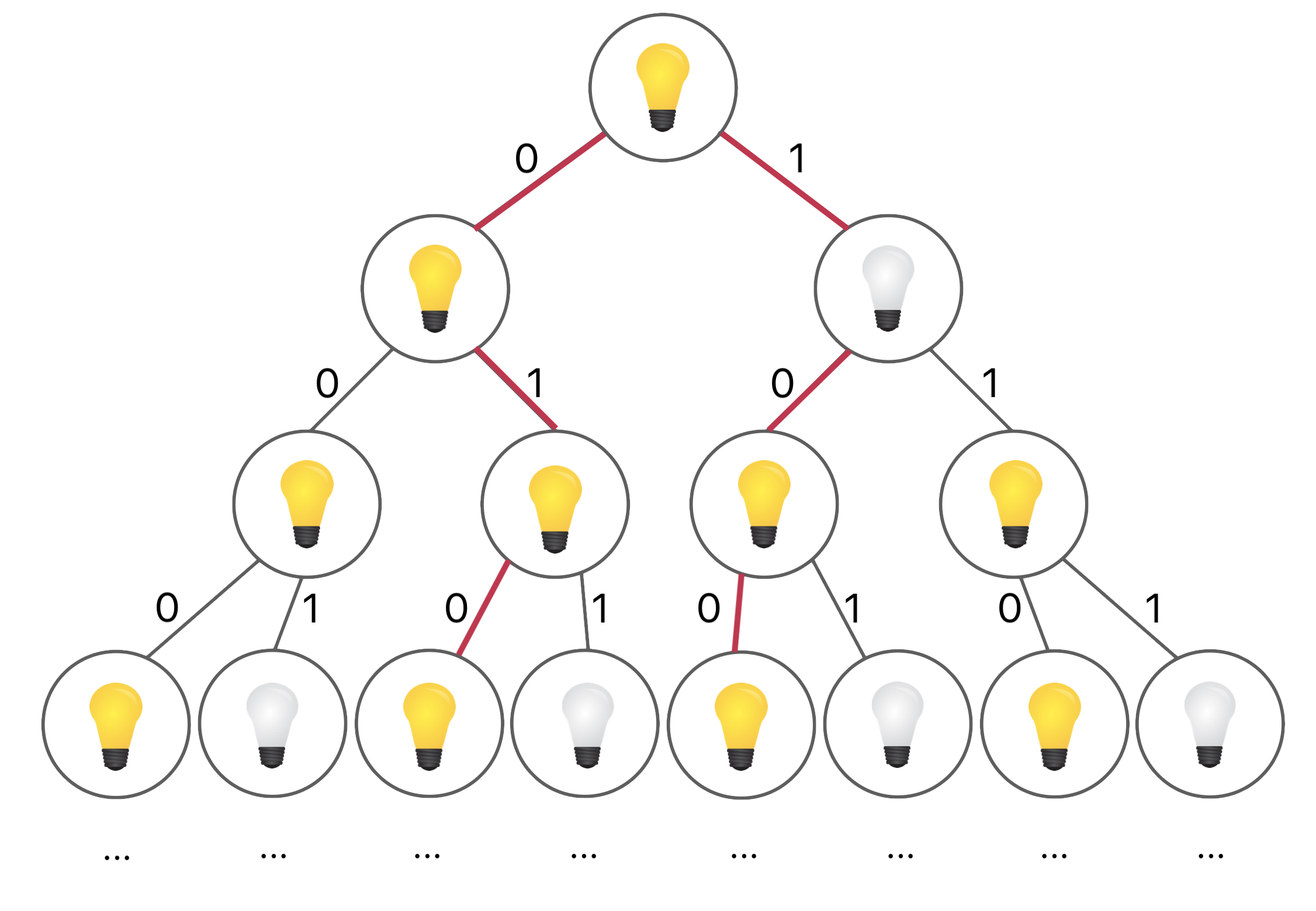
The two red marked traces are different since they differ in
the second state. this proves, that not all traces are the
same and
therefore the
light behaves different depending on the input. But we do
not have to think about a counter example ourselves. The
tool already provided a counter example. So let's have a
closer look at it. The counter example gives us an
assignment for the parameters in the system. We
have already learned that for every
quantifier the system is copied once and therefore the
parameter in_0 then refers to the parameter
in in the system copy 0. The
term in_0@0 = 0 then means that this
parameter is set to 0 at the
time step 0. The counter example states the
assignment in_0@0 = 0 and
in_1@0 = 1. That means, that we choose the
left directory for the first trace and the right directory
for the other trace. These decisions then lead to states where
the light does not behave the same. Therefore we have already
found a violation to our property.
We have seen a system, that does not fulfill the property - you could say that this system contained a bug because it does not match its specification. Instead, a system that has the following traces, would satisfy the property:

We now have to adjust our previous system in order to remove the bug. An automaton that has exactly these traces can look like this:
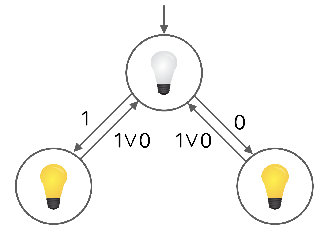
In this automaton, we can already see, that it does not matter which input we provide, the light will always behave the same way. It is worth noting, that the automaton could be simplified and would still accept the same inputs. However, we chose this example because it has a closer relation to the first automaton. A Verilog realization of this automaton is:
The complete working example can be found in the interactive tool below:
When running the tool with the corrected example, the tool
confirms that
the property holds for the system: Property proved.
Counter-example is
not available. is printed to the
Console.
In this example we have a closer look at the exists quantifier and its specialities. Let's use the system from the first example again:
Assuming we want to find out if there exists a trace in this system where the light is always on we can test the system against the property:
After a short inspection, it seems obvious that there is such
a trace (for example if the input stream only contains zeros,
we always switch between the states, where the light is
on). However, if we run the tool with this input, we
encounter the message: Counterexample found.
The property surely holds for the system, so why is that
the case? This is due to the tools implementation.
Therefore the counter example does not prove the exists property wrong but serves as actual prove for the property . The example mentioned above can be experienced in the tool interface below:
This means that there can be up to one exists statement nested in a forall statement and vice versa. As example we want to verify in the following system, that for every trace there exists a trace where the light behaves exactly the opposite way.

The property is then formulated as follows:
The property states, that for every trace p
there should exist a trace q, that fulfills some
condition. Since it would be a way too hard problem to
check if there exists such a q for every
p we reduce the computational effort needed by
defining a strategy. The strategy describes how the parameter
assignment for the
system copy 1 referring to the existential quantifier must
look like depending on the parameter assignment in the system
copy 0 referring to the forall quantifier. The strategy can
be seen as a function that gets the assignment of the all
quantifier and creates an assignment for the existential
quantifier. Therefore the forall exists problem is reduced
to a forall problem that can be solved.
For our example we need to decide, which direction we need
to take for trace
q when we know which direction was taken in trace
p? The answer is simple for that case: We need
to choose exactly the opposite input.
How do we realise that in our interface? We specify the
strategy in the Strategy tab as another
Verilog module. This Verilog module contains all inputs of
the system copy 0 as inputs, namely in_0, and all
inputs of the system copy 1 as outputs, namely
in_1. Then we assign in_1 the
negated value of in_0 and we are done.
The strategy in the forall exists case can be seen as "smart black box" playing a simple decision based game. Its target is to always choose the right direction for the trace referring to the existential quantifier as reaction to the direction chosen by the trace referring to the forall quantifier.
The complete example can be experienced in the interface below:
For the opposite case, the exists forall alternation, we also define a strategy for trace referring to the existential quantifier. But in this case we do not need to choose the assignment of the existential quantifier in dependeny of the forall quantifier. Instead we just provide an assignment for the existential quantifier. Therefore the Verilog module for the strategy would not contain any input but only outputs.
With the strategy approach mentioned in the last section there is
one remaining problem: we are not complete. This means that there
are properties that are satisfiable but that we can not prove. This
can be the case for properties like
forall p. exists q. (light_q <-> X light_p). So
why can we not decide about strategies like this
one? To do so we need knowledge about the future to define a
strategy for the assignment of the existential quantifier since
there is an comparison including different time steps.
Fortunately there is a way to fix this: prophecy variables. What
is a
prophecy
variable? We assume that we can guess the value for
X light_p and this guess is then stored in a
variable v, the prophecy variable. Now we change the
formula above to
the following: forall p. exists q. (v_p <-> X
light_p) ->
(light_q <-> X light_p). We need to assign v
to some trace and in this case we chose p. In
the case
that we guess the value for
X light_p correctly, we are able to decide
the original formula since we then can use v in the
strategy for the existential quantifier and do not need to
have knowledge about the future.